Welcome
This is a demo on how we may publish a notebook from DataLabs, with data, packages, and workflow pre-loaded in a coding envrionment, accompanied by rich narratives. This notebook is a companion to the following R journal publication, where we provides details of our approach:
The source code (.Rmd) of this notebook is deposited in the NERC Environmental Information Data Centre (EIDC). Please cite it when you are referring to the app:
![]()
This example is derived from an academic paper I have submitted that is currently under review. More information will follow.
This work is supported by:
- NERC Grant NE/T006102/1, Methodologically Enhanced Virtual Labs for Early Warning of Significant or Catastrophic Change in Ecosystems: Changepoints for a Changing Planet, funded under the Constructing a Digital Environment Strategic Priority Fund.
- Additional support is provided by the UK Status, Change and Projections of the Environment (UK-SCAPE) programme started in 2018 and is funded by the Natural Environment Research Council (NERC) as National Capability (award number NE/R016429/1).
- The initial development work of DataLabs was supported by a NERC Capital bid as part of the Environmental Data Services (EDS).
The solution proposed is to redner the Rmarkdown notebook as an R Shiny site. Specifically, it is to render the R markdown document as a Shiny prerendered document with the learnr package. This package was designed for interactive online tutorials, with ‘sandboxes’ (i.e. executable code boxes) to allow users to type in their code, which they can run it and check answers. We can pre-filled the ‘sandboxes’ with parts of the published workflow and their outputs (and linked different parts if one depends on another). And with the ‘start over’ button, the pre-filled published workflow will re-appear.
Here are some of the advantages:
- No change to the normal workflow to work with R markdown documents. Only need to supply a few extra code chunk options. Minimal extra training for scientist already
- This makes sure the published version of the code is not altered, but users can tweek it in a contained way (changes does not affect beyond each sandbox during each session).
- This is a more contained approach than the Jupyter/BinderHub/Colab approach, where users can change the entire notebook . Our approach makes sure the narrative and any bits of codes we don’t want the user to change (e.g. the
setupchunk) cannot be changed. It gives more structure and the user can reset a ‘sandbox’ rather than the entire notebook if they want to see what’s done in the published version. - This is less involved than writing a full-on Shiny app. No need to worry much about UI appearance and reactivity.
- DataLabs already has the capability to publish Shiny sites. This approach requires only minor re-configuration on DataLabs.
- Currently, DataLabs publish Shiny sites by making a copy from the directory of the Shiny app to a separate container. So all the required packages (right versions), data, and scripts will be most up to date.
Example application
The goal of our approach helps users to reproduce elements of a research workflow. As a demonstrator, this app allows users to reproduce elements (e.g. figures) of our paper ‘Rainfall and weather type effects on atmospheric deposition chemistry in the British Isles (1993 – 2015) and the potential influence of climate change’, which is currently under review.
Setup
I have preloaded the following datasets, packages, and scripts. Note that only the setup chunk in the Rmd document can be called by other code chunks by default. Future releases of learnr should allow better linking of outputs between chunks.
This code chunk reads all the required datasets and define functions to be used, which includes:
- Reading ECN rainfall chemistry data
- Reading ECN weather data
- Reading ERA5 weather reanalysis data
- Reading daily Lamb weather type data
- Reading daily Atlantic multidecadal oscillation (AMO) data
- Various functions to read, aggregate, and transform data in a usable form
# https://beta.rstudioconnect.com/content/2671/Combining-Shiny-R-Markdown.html
library(learnr)
tutorial_options(exercise.timelimit = 60,
                 exercise.completion=TRUE,
                 exercise.eval=TRUE)
knitr::opts_chunk$set(
  tidy = FALSE
)

library(ncdf4)
library(lubridate)
library(plotly)
library(ggplot2)
library(lubridate)
library(stringr)
library(cowplot)
library(dplyr)
library(changepoint)
library(feather)
library(stringi)
library(stringr)
library(readr)
library(tidyr)
library(maps)
library(here)
library(ggrepel)

# color blind friendly palette (with grey):
cbf_1 <- c("#999999", "#E69F00", "#56B4E9", "#009E73",
           "#F0E442", "#0072B2", "#D55E00", "#CC79A7")

# color_blind_friendly palette (with black):
cbf_2 <- c("#000000", "#E69F00", "#56B4E9", "#009E73",
           "#F0E442", "#0072B2", "#D55E00", "#CC79A7")

era5 = function(ncfname){
  era5_single = function(ncfname){
    ncin <- nc_open(ncfname)
    #print(ncin)
    out = tibble(t  = make_datetime(1900,1,1,ncvar_get(ncin,"time"),0,0),
                 cp = ncvar_get(ncin,"cp"),
                 lsp = ncvar_get(ncin,"lsp"),
                 lspf = ncvar_get(ncin,"lspf"),
                 ERA5_rain = ncvar_get(ncin,"tp"),)
    nc_close(ncin)
    return(out)
  }
  out = tibble()
  for (i in 1:length(ncfname)){
    out = rbind(out,era5_single(ncfname[i]))
  }

  return(out)
}

get_datechem <- function(site){
  lamb_type_lookup <-  read_csv(here('data',"lamb-type-lookup.csv"))

  lamb_data = read_csv(here('data','20CR_1871-1947_ncep_1948-2020_12hrs_UK.csv')) %>%
    dplyr::mutate(DATE = make_date(year,month,day)) %>%
    dplyr::select(DATE,LWT) %>%
    dplyr::mutate(LWT = as.character(LWT)) %>%
    dplyr::mutate(LWT = setNames(lamb_type_lookup$Type,lamb_type_lookup$Num)[LWT])


  ### get ERA5

  # files = list.files(pattern = paste0('download_',site,"_"),path = '/data/rain_pattern/ERA5',full.names = T)
  # ERA5 = era5(files) %>%
  #   mutate(cp = 1000*cp, lsp = 1000*lsp,ERA5_rain =cp+lsp, frac = cp/ERA5_rain) %>%  # m to mm
  #   group_by(date(t)) %>%
  #   mutate(frac_daily = mean(frac)) %>%
  #   ungroup() %>%
  #   mutate(frac = ifelse(!between(frac,0,1),NA,frac) ) %>%
  #   mutate(frac = ifelse(frac <1e-6,0,frac) ) %>%
  #   tidyr::fill(frac,.direction="down")

  ### get rain flux
  rain_daily = read_feather("/data/rain_pattern/rain_hourly.feather") %>%
    dplyr::filter(SITECODE == site) %>%
    dplyr::mutate(SDATE = as.Date(SDATE,format="%d-%b-%y")) %>%
    dplyr::rename(DATE = SDATE) %>%
    group_by(DATE) %>%
    summarise(VALUE = sum(VALUE))

  ### end get rain flux

  # list of PC dates that passes QC
  QC_date = readr::read_csv('/data/rain_pattern/ECN_PC_chemistry-QC.csv') %>%
    dplyr::filter(OVERALL_CHECK_OK == 1, SITECODE== site) %>%
    dplyr::rename(DATE = SDATE) %>%
    dplyr::filter(SITECODE == site) %>%
    dplyr::mutate(DATE = as.Date(DATE,format="%d-%b-%y")) %>%
    dplyr::select(DATE) %>% pull


  rain_chem = read_csv("/data/rain_pattern/ECN_PC1.csv")   %>%
    dplyr::rename(DATE = SDATE) %>%
    dplyr::filter(SITECODE == site) %>%
    dplyr::filter(!FIELDNAME %in% c("VACUUM","PHAQCS","PHAQCU")) %>%  ## remove variables
    dplyr::filter(!str_detect(FIELDNAME, "Q"))    %>%
    #dplyr::mutate(FIELDNAME = paste(FIELDNAME,"(Rain)")) %>%
    dplyr::mutate(DATE = as.Date(DATE,format="%d-%b-%y"))

  # outlier removal, note 1 mg/L to 1ppm
  # http://inside.mines.edu/~epoeter/_GW/resultsNOV03.pdf
  rain_chem = rain_chem %>%
    tidyr::spread(FIELDNAME,VALUE) %>%
    #dplyr::filter(!PO4P > 1.0) %>%
    #dplyr::filter(between( (SODIUM/23)/(CHLORIDE/35.5), 0.8,1.2)) %>% # seasalt check
    dplyr::mutate(`non-marine sulphate` = (SO4S*3*20.83-28.21*0.104*CHLORIDE)/1000 ) %>% # in meq/L
    dplyr::mutate(#ALKY = ALKY/61, # as for Hco3, everything to meq/L
      H = 10^(6-PH)/1000, # ph to meq/L
      ALUMINIUM=ALUMINIUM/26.98*3,
      CALCIUM=CALCIUM/40.08*2,
      CHLORIDE=CHLORIDE/35.45,
      IRON=IRON/55.845*2,
      MAGNESIUM=MAGNESIUM/24.3*2,
      POTASSIUM=POTASSIUM/39.1,
      SODIUM=SODIUM/22.99,
      NH4N=NH4N/14.01,
      NO3N=NO3N/14.01,
      PO4P=PO4P/15,
      SO4S=SO4S*3/96*2,
      EC=(H*349.8+SO4S*79.8+NO3N*71.4+NH4N*73.5+SODIUM*50.1+
            MAGNESIUM*53.05+CALCIUM*59.5+CHLORIDE*76.4+POTASSIUM*73.5), # tehorectical EC based on diffusion coefficient (Nernst-Einstein Equation),https://www.aqion.de/site/77
      EC_ratio = CONDY/EC,
      EC_balance = (CONDY-EC)/(CONDY+EC)
    ) %>%  # convert all ions to meq/L
    dplyr::mutate(sum_anion = CHLORIDE+NO3N+PO4P+SO4S,
                  sum_cation= NH4N+CALCIUM+MAGNESIUM+POTASSIUM+SODIUM,
                  charge_balance = (sum_cation-sum_anion)/(sum_cation+sum_anion)) %>%
    #dplyr::filter(!abs(charge_balance) > 0.05) %>%
    #dplyr::filter(!abs(EC_balance) > 0.2) %>%  # measured TDS/ theorectical TDS should be between 1.0 and 1.2
    tidyr::gather(FIELDNAME,VALUE,-SITECODE,-DATE) %>%
    dplyr::filter(DATE %in% QC_date)


  # convert all ions to meq/L

  date_chem = distinct(rain_chem,DATE) %>%
    dplyr::arrange(DATE) %>%
    dplyr::mutate(SDATE = as.Date(DATE,format="%d-%b-%y")) %>%
    dplyr::mutate(DIFF = as.numeric(difftime(DATE,lag(DATE,1)))) %>%
    dplyr::mutate(STARTDATE = lag(DATE,1)+1, ENDDATE = DATE) %>%
    dplyr::filter(!is.na(DIFF)) %>%
    dplyr::filter(between(DIFF,6,8)) #%>%
  #dplyr::mutate(lamb_str2 = NA,mean_rain_per_day = NA) # maximum len of continuous rain > 0.1


  get_lamb_str2 <- function(lamb_data,STARTDATE,ENDDATE){
    lamb_data %>%
      filter(between(DATE,STARTDATE,ENDDATE)) %>%
      select(LWT) %>%
      mutate(LWT = case_when(LWT == "C" | LWT == "W" |
                               LWT == "SW" |LWT == "CW" |
                               LWT == "CSW"  ~ "1" , TRUE ~ "0")) %>% #event generating types
      pull() %>% paste(collapse = '')
  }
  get_lamb_strW <- function(lamb_data,STARTDATE,ENDDATE){
    lamb_data %>%
      filter(between(DATE,STARTDATE,ENDDATE)) %>%
      select(LWT) %>%
      mutate(LWT = case_when(LWT == "W" |LWT == "SW" |LWT == "CW" |LWT == "CSW"  ~ "1" ,
                             TRUE ~ "0")) %>% #event generating types
      pull() %>% paste(collapse = '')
  }
  get_lamb_strC <- function(lamb_data,STARTDATE,ENDDATE){
    lamb_data %>%
      filter(between(DATE,STARTDATE,ENDDATE)) %>%
      select(LWT) %>%
      mutate(LWT = case_when(LWT=="C"|LWT=="CSW" |LWT=="CW"|LWT=="CNW"|LWT=="CN"|
                               LWT=="CNE"|LWT=="CE"|LWT=="CSE"|LWT=="CS"  ~ "1" ,
                             TRUE ~ "0")) %>% #event generating types
      pull() %>% paste(collapse = '')
  }

  date_chem = date_chem %>%
    rowwise() %>%
    mutate(lamb_str2= get_lamb_str2(get("lamb_data"),STARTDATE,ENDDATE),
           lamb_strW= get_lamb_strW(get("lamb_data"),STARTDATE,ENDDATE),
           lamb_strC= get_lamb_strC(get("lamb_data"),STARTDATE,ENDDATE),
           mean_rain_per_day = filter(rain_daily,between(DATE,STARTDATE,ENDDATE)) %>%
             select(VALUE) %>% pull() %>% mean(na.rm=T),
           #cp_week=filter(ERA5,between(`date(t)`,STARTDATE,ENDDATE)) %>% select(cp) %>% sum(),
           #era5_week = filter(ERA5,between(`date(t)`,STARTDATE,ENDDATE)) %>% select(ERA5_rain) %>% sum()
    ) %>%
    ungroup()

  date_chem = date_chem %>% mutate(SITECODE=site) %>% select(-SDATE,-STARTDATE,-ENDDATE) %>%
    left_join(rain_chem %>% select(-SITECODE) %>% tidyr::spread(FIELDNAME,VALUE), by="DATE") %>%
    gather(FIELDNAME,VALUE,-DATE,-DIFF,-lamb_str2,-lamb_strW,-lamb_strC,-SITECODE,-mean_rain_per_day,
           #-cp_week,-era5_week,
           -VOLUME)

  print(paste0('Complete ',site,'!'))


  return(date_chem)
}


data0 = rbind(get_datechem('T02'),get_datechem('T04'),get_datechem('T06'),get_datechem('T11'))
## [1] "Complete T02!"
## [1] "Complete T04!"
## [1] "Complete T06!"
## [1] "Complete T11!"date_chem = data0 %>%
tidyr::spread(FIELDNAME,VALUE) %>%
mutate(SITECODE = case_when(
SITECODE == 'T02' ~ 'Glensaugh',
SITECODE == 'T04' ~ 'Moor_House',
SITECODE == 'T06' ~ 'Rothamsted',
SITECODE == 'T01' ~ 'Drayton',
SITECODE == 'T07' ~ 'Sourthrope',
SITECODE == 'T11' ~ 'Snowdon',
TRUE ~ SITECODE
)) %>%
mutate(lamb2count=sapply(strsplit(lamb_str2, ''), function(x) sum(as.numeric(x))) ,
lambCcount=sapply(strsplit(lamb_strC, ''), function(x) sum(as.numeric(x))) ,
lambWcount=sapply(strsplit(lamb_strW, ''), function(x) sum(as.numeric(x))) ,
yr_grp = case_when(
between(year(DATE),1992,1995) ~ '1992-1995',
between(year(DATE),1996,1999) ~ '1996-1999',
between(year(DATE),2000,2003) ~ '2000-2003',
between(year(DATE),2004,2007) ~ '2004-2007',
between(year(DATE),2008,2011) ~ '2008-2011',
between(year(DATE),2012,2015) ~ '2012-2015',
TRUE ~ NA_character_),
lamb_grp2 = case_when(
between(lamb2count,0,2) ~ '0-2',
#between(lamb2count,2,3) ~ '2-3',
# between(lamb2count,3,3) ~ '3',
# between(lamb2count,4,4) ~ '4',
between(lamb2count,3,5) ~ '3-5',
between(lamb2count,6,8) ~ '6 or more',
TRUE ~ NA_character_),
lambCcountgrp = case_when(
between(lambCcount,0,1) ~ '0-1',
between(lambCcount,2,3) ~ '2-3',
between(lambCcount,4,5) ~ '4-5',
between(lambCcount,6,8) ~ '6 or more',
TRUE ~ NA_character_),
lambWcountgrp = case_when(
between(lambWcount,0,1) ~ '0-1',
between(lambWcount,2,3) ~ '2-3',
between(lambWcount,4,5) ~ '4-5',
between(lambWcount,6,8) ~ '6 or more',
TRUE ~ NA_character_),
# conv3grp = case_when(
# between(cp_week/era5_week,0,0.2) ~ '0-20%',
# between(cp_week/era5_week,0.2,0.5) ~ '20-50%',
# between(cp_week/era5_week,0.5,0.8) ~ '50-80%',
# between(cp_week/era5_week,0.8,1.0) ~ '80-100%',
# TRUE ~ NA_character_),
season = case_when(
month(DATE) %in% 3:5 ~ 'Spring (MAM)',
month(DATE) %in% 6:8 ~ 'Summer (JJA)',
month(DATE) %in% 9:11 ~ 'Autumn (SON)',
month(DATE) %in% c(12,1,2) ~ 'Winter (DJF)',
TRUE ~ NA_character_),
season = factor(season,levels=c('Spring (MAM)','Summer (JJA)','Autumn (SON)','Winter (DJF)')),
#wm = weighted.mean(VALUE,VOLUME)
) #%>%
#ungroup() %>%
# filter(!(FIELDNAME == 'CONDY' & VALUE > 100)) %>%
# filter(!(FIELDNAME == 'NO3N' & VALUE > 5)) %>%
# filter(!(FIELDNAME == 'NH4N' & VALUE > 5)) %>%
# filter(!(FIELDNAME == 'CHLORIDE' & VALUE > 7.5)) %>%
# filter(!(FIELDNAME == 'SODIUM' & VALUE > 5)) %>%
# filter(!(FIELDNAME == 'non-marine sulphate' & VALUE > 50)) %>%
#filter(!(VALUE < 0))
date_chem = date_chem %>%
mutate(SODIUM=SODIUM*1000, CHLORIDE=CHLORIDE*1000, NH4N=NH4N*1000,
NO3N=NO3N*1000, `non-marine sulphate`=`non-marine sulphate`*1000)
# date_chem = date_chem %>% group_by(SITECODE) %>%
# mutate(conv3quant = rank(cp_week/era5_week)/length(cp_week/era5_week)) %>%
# mutate( conv3grp = case_when(
# between(conv3quant,0,0.33) ~ '0-33%',
# between(conv3quant,0.33,0.67) ~ '33-67%',
# between(conv3quant,0.67,1.0) ~ '67-100%',
# TRUE ~ NA_character_))Figure 1: ECN map
This code plots the map of selected ECN stations.
# draw ECN map
library(maps)

library(ggrepel)
UK <- map_data("world") %>% filter(region=="UK")
Ireland <- map_data("world") %>% filter(region=="Ireland")
IoM <- map_data("world") %>% filter(region=="Isle of Man")
data <- world.cities %>% filter(country.etc=="UK")

# 4 ECN sites
ECN_site_info <- data.frame(
  "sitecode" = 1:12,
  "name" = c("Drayton","Glensaugh","Hillsborough","Moor House",
             "North Wyke","Rothamsted","Sourhope","Wytham",
             "Alice Holt","Porton Down","Snowdon","Cairngorms"),
  "lat" = c(52.193875,56.9092667,54.4534,54.6950416666,
            50.781933335,51.803425,55.4898527778,51.781349999999996,
            51.15457222,51.127175,53.07455,57.11634444),
  "long" = c(-1.764430555,-2.55337222,-6.0781277778,-2.38785,
             -3.91780555553,-0.372683333,-2.2120333,-1.3360583333333333,
             -0.86321666,-1.63985,-4.03351111,-3.82971667))

ECN_site_info <-ECN_site_info[c(2,4,6,11),]
ggplot() +
  geom_polygon(data = UK, aes(x=long, y = lat, group = group), fill="darkgrey", alpha=0.7) +
  geom_polygon(data = Ireland, aes(x=long, y = lat, group = group), fill="grey", alpha=0.5) +
  geom_polygon(data = IoM, aes(x=long, y = lat, group = group), fill="grey", alpha=0.3) +
  #geom_point( data=data, aes(x=long, y=lat, alpha=pop)) +
  geom_text_repel( data=ECN_site_info, aes(x=long, y=lat, label=name), size=5) +
  geom_point( data=ECN_site_info, aes(x=long, y=lat), color="red", size=3) +
  theme_void() + ylim(50,61) + coord_map() +
  theme(legend.position="none")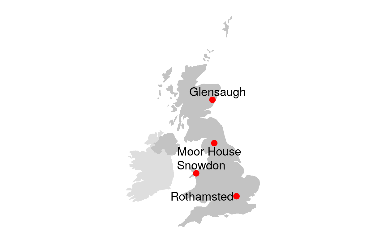
Figure 1: ECN map (with selectors)
This code is a duplicate of the previous one. However, R Shiny selectors are added for easier site selection.
Figure 2: Lamb cyclones/westerlies counts (1871-2020)
This plots the yearly Lamb cyclones/westerlies counts (1871-2020). The top graph fits a changepoint alogorithm to it, while the seconds shows the second derivative of its deviation from mean, as well as overlaying the Atlantic multidecadal oscillation (AMO).
source(here('R','cpt_helpers.R'))
source(here('R','Deriv.R'))
library(mgcv);
Loading required package: nlme
Attaching package: 'nlme'The following object is masked from 'package:dplyr':
collapseThis is mgcv 1.8-27. For overview type 'help("mgcv-package")'.lamb_type_lookup <- read_csv(here("data","lamb-type-lookup.csv")) ;
── Column specification ────────────────────────────────────────────────────────
cols(
  Num = col_double(),
  Type = col_character()
)
lamb_data = read_csv(here('data','20CR_1871-1947_ncep_1948-2020_12hrs_UK.csv')) %>%
dplyr::mutate(DATE = make_date(year,month,day)) %>%
dplyr::select(DATE,LWT) %>%
dplyr::mutate(LWT = as.character(LWT)) %>%
dplyr::mutate(LWT = setNames(lamb_type_lookup$Type,lamb_type_lookup$Num)[LWT]);
── Column specification ────────────────────────────────────────────────────────
cols(
  day = col_double(),
  month = col_double(),
  year = col_double(),
  PM_1000 = col_double(),
  w = col_double(),
  s = col_double(),
  f = col_double(),
  z = col_double(),
  g = col_double(),
  dir = col_double(),
  LWT = col_double()
)
currData = lamb_data %>% mutate(wk_year=(yday(DATE)-1)%/%7 + 1, yday = yday(DATE),year=year(DATE),
lamb_grp2= case_when(
LWT %in% c('C','W','SW','CW','CSW') ~ "(C,W,SW,CW,CSW)",
TRUE ~ "others")) %>%
group_by(year)%>%
filter(lamb_grp2 == "(C,W,SW,CW,CSW)") %>%
summarise(N = n());
cpt.mean(currData$N,penalty="Manual",pen.value=0.8,method="AMOC",test.stat="CUSUM");Class 'cpt' : Changepoint Object
~~ : S4 class containing 12 slots with names
cpttype date version data.set method test.stat pen.type pen.value minseglen cpts ncpts.max param.est
Created on : Fri Apr 23 10:17:37 2021
summary(.) :
----------
Created Using changepoint version 2.2.2
Changepoint type : Change in mean
Method of analysis : AMOC
Test Statistic : CUSUM
Type of penalty : Manual with value, 0.8
Minimum Segment Length :
Maximum no. of cpts : 1
Changepoint Locations : 41 out=cpt.meanvar(currData$N,pen.value=c(2*log(length(currData$N)),100*log(length(currData$N))),penalty="CROPS",method="PELT",test.stat = "Poisson");[1] "Maximum number of runs of algorithm = 7"
[1] "Completed runs = 2"
[1] "Completed runs = 3"
[1] "Completed runs = 5"
[1] "Completed runs = 6"currData = currData %>% rename(value=N) %>% mutate(segment = 1);
for (ii in 1:length(!is.na(out@cpts.full[1,]))) {
if (ii == length(!is.na(out@cpts.full[1,]))) {
currData$segment[out@cpts.full[1,ii]: length(out@data.set)] = ii+1
}else {
currData$segment[out@cpts.full[1,ii]:out@cpts.full[1,ii+1]] = ii + 1
}
};
currData = currData %>% group_by(segment) %>% mutate(mean=mean(value),var=var(value),meanGroup=segment,varGroup=segment);
p1 = createChangePointPlot('cpt.meanvar', currData %>% mutate(temporalField = make_date(year,1,1))) +
labs(title = paste0('Number of Lamb westerlies/cyclones days per year (1871-', max(currData$year) ,')'),
subtitle = "Changepoints using cpt.meanvar (pentaly = 'CROPS',method='PELT',test.stat='Poission')" #,
# caption = "Data source: Climate Research Unit"
) + ylab('count') + xlab('Year') +
theme_half_open(12) +
background_grid(major = 'y', minor = "none") +
panel_border() + background_grid();# A tibble: 6 x 8
# Groups: segment [2]
year value segment mean var meanGroup varGroup temporalField
<dbl> <int> <dbl> <dbl> <dbl> <dbl> <dbl> <date>
1 1871 126 1 152. 914. 1 1 1871-01-01
2 1872 185 1 152. 914. 1 1 1872-01-01
3 1873 144 1 152. 914. 1 1 1873-01-01
4 1874 141 2 128. 237. 2 2 1874-01-01
5 1875 110 2 128. 237. 2 2 1875-01-01
6 1876 110 2 128. 237. 2 2 1876-01-01 AMO = read_csv(here('data','AMO_smoothed_from_the_Kaplan_SST_V2.csv')) %>%
gather(key="month",value="value",-Year) %>%
mutate(month= match(month,toupper(month.abb)), Date = make_date(Year,month,1)) %>%
select(-Year,-month) %>%
filter(!value < -99) %>%
mutate(year=year(Date)+yday(Date)/366);
── Column specification ────────────────────────────────────────────────────────
cols(
  Year = col_double(),
  JAN = col_double(),
  FEB = col_double(),
  MAR = col_double(),
  APR = col_double(),
  MAY = col_double(),
  JUN = col_double(),
  JUL = col_double(),
  AUG = col_double(),
  SEP = col_double(),
  OCT = col_double(),
  NOV = col_double(),
  DEC = col_double()
)
lamb_type_lookup <- read_csv(here('data',"lamb-type-lookup.csv")) ;
── Column specification ────────────────────────────────────────────────────────
cols(
  Num = col_double(),
  Type = col_character()
)
lamb_data = read_csv('/data/rain_pattern/20CR_1871-1947_ncep_1948-2020_12hrs_UK.csv') %>%
dplyr::mutate(DATE = make_date(year,month,day)) %>%
dplyr::select(DATE,LWT) %>%
dplyr::mutate(LWT = as.character(LWT)) %>%
dplyr::mutate(LWT = setNames(lamb_type_lookup$Type,lamb_type_lookup$Num)[LWT],
season = case_when(
month(DATE) %in% 3:5 ~ 'Spring (MAM)',
month(DATE) %in% 6:8 ~ 'Summer (JJA)',
month(DATE) %in% 9:11 ~ 'Autumn (SON)',
month(DATE) %in% c(12,1,2) ~ 'Winter (DJF)',
TRUE ~ NA_character_));
── Column specification ────────────────────────────────────────────────────────
cols(
  day = col_double(),
  month = col_double(),
  year = col_double(),
  PM_1000 = col_double(),
  w = col_double(),
  s = col_double(),
  f = col_double(),
  z = col_double(),
  g = col_double(),
  dir = col_double(),
  LWT = col_double()
)
currData = lamb_data %>% mutate(wk_year=(yday(DATE)-1)%/%7 + 1, yday = yday(DATE),year=year(DATE),
lamb_grp2= case_when(
LWT %in% c('C','W','SW','CW','CSW') ~ "(C,W,SW,CW,CSW)",
TRUE ~ "others")) %>%
group_by(year)%>%
filter(lamb_grp2 == "(C,W,SW,CW,CSW)") %>%
summarise(N = n());
#### FIT ADDITIVE MODEL
ctrl <- list(niterEM = 0, msVerbose = TRUE, optimMethod="L-BFGS-B");
m2 <- gamm(N ~ s(year, k =9),
data = currData,
control = ctrl); 0: 800.09450: -0.754777
1: 799.74261: -1.33589
2: 799.57216: -3.66032
3: 799.27010: -2.28271
4: 799.19555: -2.64645
5: 799.19137: -2.77221
6: 799.19121: -2.75142
7: 799.19120: -2.75207
8: 799.19120: -2.75209want <- seq(1, nrow(currData), length.out = 200);
pdat <- with(currData, data.frame(year = year[want]) );
p2 <- predict(m2$gam, newdata = pdat, type = "terms", se.fit = TRUE);
pdat <- transform(pdat, p2 = p2$fit[,1], se2 = p2$se.fit[,1]);
df.res <- df.residual(m2$gam);
crit.t <- qt(0.025, df.res, lower.tail = FALSE);
pdat <- transform(pdat,
upper = p2 + (crit.t * se2),
lower = p2 - (crit.t * se2));
Term <- "year";
m2.d <- Deriv(m2);
m2.dci <- confint(m2.d, term = Term);
m2.dsig <- signifD(pdat$p2, d = m2.d[[Term]]$deriv,
m2.dci[[Term]]$upper, m2.dci[[Term]]$lower);
p2=ggplot(pdat) +
geom_line(data=AMO,aes(x=year,y=value*100),col='firebrick4')+
geom_area(data=AMO,aes(x=year,y=value*100),fill='firebrick4',alpha=0.2,col=NA)+
geom_line(aes(year,p2))+
geom_line(aes(year,lower),linetype='dashed')+geom_line(aes(year,upper),linetype='dashed')+
geom_line(aes(year,unlist(m2.dsig$incr)), col='blue', size=2 )+
geom_line(aes(year,unlist(m2.dsig$decr)), col='red', size=2 )+
ylab('count anomaly or AMO (x100)')+ xlab('Year') +
theme_half_open(12) +
background_grid(major = 'y', minor = "none") +
panel_border() + background_grid()+
ggtitle('Lamb cyclones/westerlies days count fitted anomaly (1871-2020)\nand Atlantic multi-decadal oscillation (AMO)');
pALL = plot_grid(p1,p2,labels = "AUTO", align = 'h', axis = "tb",nrow = 2);
pALL;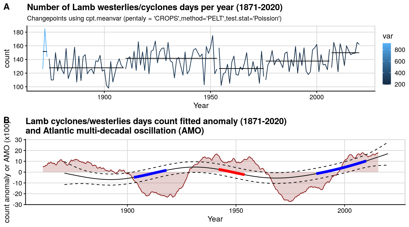
#save_plot(paste0("lamb_1871_2020.png"), pALL, base_height =NULL, base_width = 7.5, dpi=128) # 714 x 660Figure 3: Lamb vs chemistry boxplots
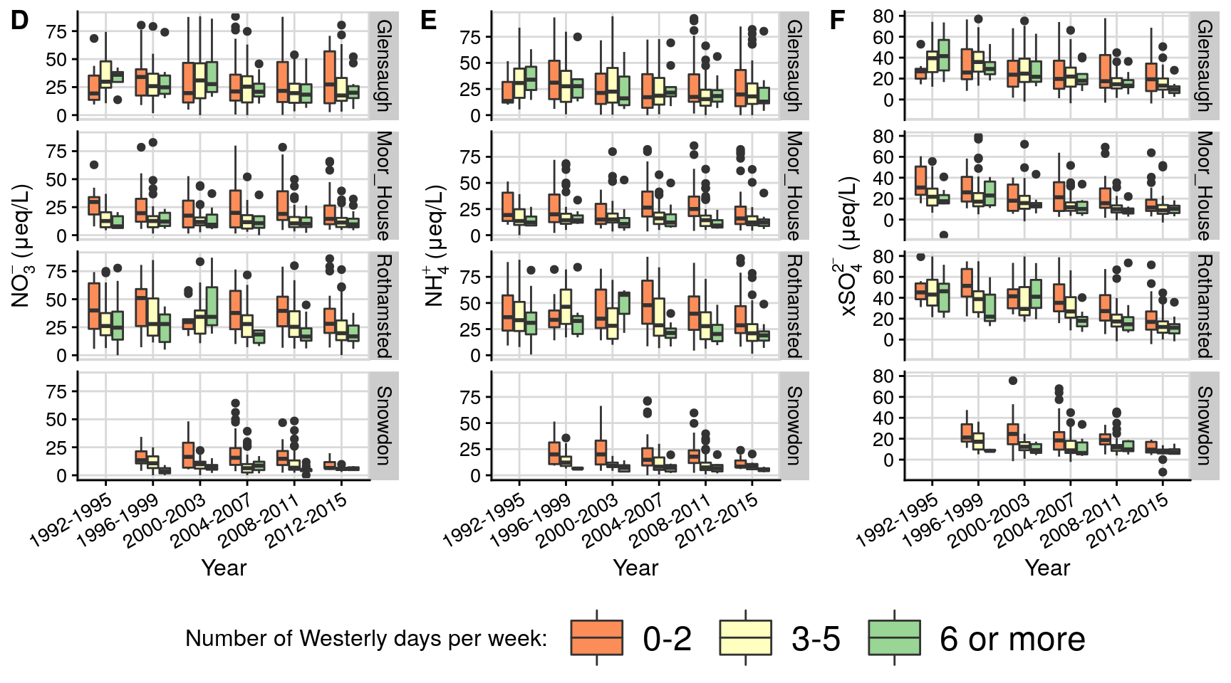
This code plots concentration over time for selected chemical species across ECN sites grouped by number of Lamb westerlies and cyclones per week. Chemical samples are taken weekly.
plot_chembox = function(date_chem, FIELDNAME,grp_name,flux=FALSE,skip_legend=1){

  if(flux==FALSE){
    y = date_chem[[FIELDNAME]]
  } else {
    y = date_chem[[FIELDNAME]]*date_chem[['VOLUME']]/1000/(pi*(0.152/2)^2)*(365.25/7) # per area per year
  }

  out = ggplot(date_chem, #%>% filter(!is.na(get(FIELDNAME))),
               #aes(x=yr_grp, y=get(FIELDNAME)*VOLUME, fill=get(grp_name))) +
               aes(x=yr_grp, y= !!y, fill=get(grp_name))) +
    geom_boxplot()+
    facet_grid(SITECODE ~ .) +
    theme_half_open(12) +
    background_grid(major = 'y', minor = "none") +
    panel_border() + background_grid()+
    scale_fill_brewer(palette = 'Spectral')+
    theme(axis.text.x=element_text(angle=30, hjust=1))+
    scale_y_continuous(limits = quantile(y, c(0., 0.95),na.rm=TRUE))

  if(skip_legend == 1){
    out = out + theme(legend.position = "none")
  }else{
    out = out +  theme(legend.position = "bottom",legend.justification = 'center',
                     legend.key.size=unit(36,units = "points") ,
                     legend.text = element_text(size = 18))
  }
  return(out)
}

grp_name = 'lamb_grp2'

p1 = plot_chembox(date_chem, "CONDY","lamb_grp2") + xlab('Year')+ylab('Electrical Conductivity (\u03BCS/cm)')
p4 = plot_chembox(date_chem, "NO3N","lamb_grp2") + xlab('Year')+ylab( expression("NO"[3]^-{}*" (\u03BCeq/L)"))
p5 = plot_chembox(date_chem, "NH4N","lamb_grp2") + xlab('Year')+ylab( expression("NH"[4]^+{}*" (\u03BCeq/L)"))+
  theme(legend.position = "bottom",legend.justification = 'center',
        legend.key.size=unit(36,units = "points") ,
        legend.text = element_text(size = 18)) +
  guides(fill=guide_legend("Number of Westerly days per week: " ))
p2 = plot_chembox(date_chem, "CHLORIDE","lamb_grp2") + xlab('Year')+ylab( expression("Cl"[]^-{}*" (\u03BCeq/L)"))+
  theme(legend.position = "bottom",legend.justification = 'center',
        legend.key.size=unit(36,units = "points") ,
        legend.text = element_text(size = 18)) +
  guides(fill=guide_legend("Number of Westerly days per week: " ))
p3 = plot_chembox(date_chem, "SODIUM","lamb_grp2") + xlab('Year')+ylab( expression("Na"[]^+{}*" (\u03BCeq/L)"))
p6 = plot_chembox(date_chem, "non-marine sulphate","lamb_grp2") + xlab('Year')+ylab( expression("xSO"[4]^2^-{}*" (\u03BCeq/L)"))

pALL = plot_grid(p1,p2,p3,labels = "AUTO", align = 'h', axis = "tb",nrow = 1)
pALL;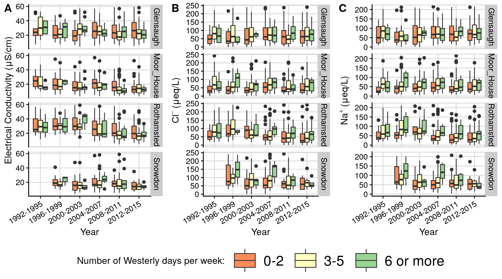
pALL = plot_grid(p4,p5,p6,labels = c("D","E","F"), align = 'h', axis = "tb",nrow = 1)
pALL